このページは、令和2年4月27日に一部更新しました。
![]()
| 反復測度 SPF-p.q デザインの GMANOVA 分析用 プログラムの例 |
この節では、SAS/IML による反復測度 SPF-p.q デザインの GMANOVA 分析の ためのプログラム例を示す。データは、前節で引用した O'Brien らの反復測度 SPF-3.3 デザインデータを用いる。
前節でもふれたように、彼らのデータは非釣り合い型デザインなので、SAS の 4つの平方和のうちの Type III よりも Type II の方がよいと考えられるが、前節 と同様にここでも Type III 平方和による方式で実行する場合の例を示す。
以下の IML プログラムからわかるように、実は通常の GMANOVA で主効果なり 同時検定に際して用いられる (1.192) 式や (1.207) 式で定義されている行列 F の内容を検討すると、反復測度の主効果を見るための (1.192) 式の F の右辺のうち、(A1t ,A1))-1 及び A1t,Y は、SPF-I.J デザインでは、A1 が、
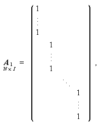
|
(1.240) |

|
(1.241) |

|
(1.242) |
となる。ここで、(1.242) 式の要素  は、第 i 独立測度
グループで第 j 反復測度変数のデータの和である。したがって、(1.193)
式の右辺の行列 C1 がこの場合、
は、第 i 独立測度
グループで第 j 反復測度変数のデータの和である。したがって、(1.193)
式の右辺の行列 C1 がこの場合、

|
(1.243) |
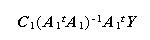
|
の第 j 列は、反復測度第 j 変数のグループごとの(単純)平均 の和になっていることがわかる。
つまり、通常の GMANOVA では、このような独立測度の水準をつぶす場合、水 準(グループ)ごとの単純平均の和を作っていることになり、水準間でサンプル数 が異なる、すなわち非釣り合い型デザインデータの場合、場合によっては都合が 悪い。これを避けるには、(1.241) 式の対角要素の値をすべて I/N にすればよい。 この操作は、独立測度の水準をつぶす場合、結局単純平均の和を作るのではなく、 各水準(グループ)のサンプル数による加重平均を考え ることに等しい。
前者と後者の平均の作り方は、SAS/STAT では平方和としてそれぞれ、Type III を 選択するか Type II を選択するかと対応している。
このようなわけで、つぎの SAS/IML プログラムでは、ユーザがこれらのうちの どちらを選択するかをユーザ自身で指定できるようにしてある(指定すべき9つの パラメータ項のうち、(d) の項)。
また、ユーザは最初、Heck チャートの3つのパラメータの値が分からないものと して、それらを打ち出すために、(i) の項の heck_c の値をゼロと指定して実行 しなければならない。これを実行し、3つのパラメータの値から Heck チャートを 見て、棄却点の値を図から読みとり、2回目のプログラム実行時には heck_c の 値をゼロから変更する必要がある。
つぎのプログラムは、(i) の項を見れば分かるように、2回目の実行時のための ものである。
*----------------------------------------------------------------------* | December 1, 1998 | | sas program--imlspfok.sas | | | | SAS/IML program for executing simultaneous contrast tests using a | | Roy-Bose simultaneous test procedure for an arbitrary repeated | | measures SPF.p-q design data. | | | | Data is Table 3, of O'Brien & Keiser (1985). | |
|  Caution!                                                            |
|                                                                      |
| (1) Users must revise the necessary parts of the following program   |
|  in order to specify (a) raw data, (b) variable names for repeated   |
|  measures, (c) levels of between-subjects factor A of all samples,   |
|  (d) type of sum of squares, (e) contrast matrix for a between-      |
|  subjects factor A, (f) names of contrasts for the between-subjecs   |
|  factor A, (g) transformation matrix for a within-subjects factor P, |
|  (h) names of contrasts for within-subjects factor P, and (i) Heck   |
|  critical value, which are suggested by the comments which  begin    |
|  with '/* Specify ... '.                                             |
| (2) Users must execute this program twice.  In the first execution,  |
|  set the heck_c value for testing the overall interaction equals to  |
|  zero.  In the second execution, specify it according to the param-  |
|  eters s_heck, m_heck, and n_heck, looking at the Heck chart.        |
| (3) It should be noticed that there is no need to specify heck_c     |
|  values for testing the two main effects.  For, test statistics be-  |
|  come exact in these cases.                                          |
| (4) Types of sum of squares (denoted by 'typess' below) must be 2 or |
|  3, which correspond to Type II SS and Type III SS in SAS anova and  |
|  glm procedures, respectively.                                       |
|                                                                      |
*----------------------------------------------------------------------*;
options pagesize=60 ls=80;

/* (1) data input */
data work;
  /* (a) Specify variable names and their labels */
  input ssno 2. +1 group 1. +1 (pretest posttest followup) (1.);
  label ssno='sample number'
        group='group number to which subject belongs'
        pretest='mark on a pretest'
        posttest='mark on a posttest'
        followup='mark on a follow-up test';
  cards;
 1 1 233
 2 1 434
 3 1 657
 4 1 534
 5 1 464
 6 2 899
 7 2 589
 8 2 356
 9 2 445
10 3 478
11 3 356
12 3 698
13 3 668
14 3 256
15 3 377
16 3 578
;
|
proc iml;
 use work;
  /* (b) Specify the variable names for repeated measures, which must
       be the same as those defined by the input statement */
 read all var{pretest posttest followup}
      into y;
 print "Input raw-data matrix, Y", y;
 yrow=nrow(y); ycol=ncol(y);

 if yrow < ycol then do;
   print "number of samples is too small"; return;
 end;

  /* (c) Specify the levels of the factor A of each sample */
   level={1,1,1,1,1,2,2,2,2,3,3,3,3,3,3,3};

  /* (d) Specify the type of sum of squares:
      (1) typess=2.....weighted average case (Type II SS in SAS glm)
      (2) typess=3.....simple average case   (Type III SS in SAS glm) */
   typess=3;

 a_1=design(level);       /* design matrix A_1 is generated */
 ata=a_1`*a_1;             /* A_1'A_1 of the design matrix A_1 */
 atai=inv(ata);

  /* (e) Specify the contrast matrix C for a between-subjects factor A */
 c_a={-2  1 1,
       0 -1 1};
  /* (f) Specify the names of contrasts for the between-subjects effect */
 name_ca={c1 c2};

  /* (g) Specify the transformation matrix M */
 m_p={-1 -1,
       1  0,
       0  1};
  /* (h) Specify the names of contrasts of P effect */
 name_mp={m1 m2};

 print "design, contrast, and transformation matrices",
               a_1, c_a, m_p;

 start test(y,yrow,a_1,c,m,atai,p,theta_h,heck_c,typess,
   namebet,namewit,namef,namedf1,namedf2,namep,namet);
   /* (1) test for overall effect */
    crow=nrow(c); ccol=ncol(c);
    mrow=nrow(m); mcol=ncol(m);
    camul=c*atai;
    if typess=2 then camul=shape(1,1,ccol)*ccol/yrow;
    f=camul*a_1`*y*m;
    contm=camul*c`;
    contmi=inv(contm);
  h=f`*contmi*f;                      /* H matrix */
    atym=a_1`*y*m;
  e=m`*y`*y*m-atym`*atai*atym;        /* E matrix */
      print h, e;
|
    call geneig(eigval,eigvec,h,e);   /* generalized eigenproblem */
  roy1=eigval[1];                     /* Roy's greatest root */
s_heck=crow> |
      end;
  end;

 finish;

 namef={F_value}; namep={Prob_ge_F}; namedf1={df_1}; namedf2={df_2};
 namet={theta_Heck};

 print "*** 1. test for the hypothesis of no interaction effect ***";
   c=c_a;   /* contrast matrix C for between-subjects levels */
   m=m_p;   /* transformation matrix M for within-subjects measures */
   namebet=name_ca;
   namewit=name_mp;

  /* (i) Specify the non-zero Heck critical value for the overall
         interaction if s_Heck is greater than 1 in the first execution
         of this program */
   heck_c=0.498;

 run test(y,yrow,a_1,c,m,atai,p,theta_h,heck_c,3,
          namebet,namewit,namef,namedf1,namedf2,namep,namet);

 print "*** 2. test for the hypothesis of no A effect ***";
   c=c_a;     /* contrast matrix C for between-subjects levels */
   mprow=nrow(m_p);
   m=shape(1,mprow,1); /* M matrix for testing A effect */
   namebet=name_ca;
   namewit={m_mean};
 run test(y,yrow,a_1,c,m,atai,p,theta_h,heck_c,3,
          namebet,namewit,namef,namedf1,namedf2,namep,namet);

 print "*** 3. test for the hypothesis of no P effect ***";
   cacol=ncol(c_a);
   c=shape(1,1,cacol); /* contrast matrix C for between-subjects levels */
   m=m_p;     /* transformation matrix M for within-subjects measures */
   namebet={c_mean};
   namewit=name_mp;
 run test(y,yrow,a_1,c,m,atai,p,theta_h,heck_c,typess,
          namebet,namewit,namef,namedf1,namedf2,namep,namet);

quit;
|
| imlspfok.sas |
![]()