第4章 MATLABやカオス時系列解析ソフトの使い方と出力例
![]()
![]()
この頁は、平成28年7月12日に新たに開設しました。
この頁は、平成30年5月24日に一部更新しました。
![]()
この節では、MATLAB ソフトの使い方と出力例を解説する。 MATLAB は、Matrix Laboratory を略したもので、伝統的なプログラミング言語である FORTRAN や BASIC 等に比べ、GUI 環境に優れたソフトである。また、MATLAB の基本演 算はスカラーではなく行列であるため、プログラミングの煩雑さが少ない。さらに、 MATLAB の基本演算は実数に対してではなく複素数であることもプログラミングの煩雑 さを少なくしている。
ここでは、MATLAB プログラムの最初の例として、音声データの解析のためのプログラム をあげる。以下の例は、澤木 (2015) が収集した音声データを MATLAB に入力し各種の (線形)時系列解析を行ったものである。まず、拡張子が mp3 である音声データを読み 込み、audioread 関数で z に掃出し、sound 関数で音声を再現する。その後、各種の 時系列解析を MATLAB に組み込まれた各種の関数を用いて実行している:
%-------------------------------------------------------------------------
%
% Program takens_sawaki_hoarse_like1.m
%
% This is a new program written by N. Chino for Sawaki's
% hoarseness-like data 1,
%       Version 1,                      written on August 16, 2015.
%
%-------------------------------------------------------------------------
fname='data/chino/Sawaki-hoarse-related/Sawaki-voice-data/sawaki-hoarse-like1.mp3';
[z,fs]=audioread(fname);
sound(z,fs);
x=z(:,1);
maxn=size(x,1);
%
tau=1;
% lowthin=1; intthin=16; upthin=maxn;
% lowthin=36002; intthin=10; upthin=134677;
% lowthin=1; intthin=16; upthin=166000;
lowthin=16000; intthin=16; upthin=166000;
%
nn=(lowthin:intthin:upthin);
xthin=x(nn);
xt=xthin;
maxt=size(xt,1);
%
% save('data/chino/Sawaki-hoarse-like1-thin16-signals.dat', 'xt', '-ASCII');
% save('data/chino/Sawaki-hoarse-like1-bothcut-thin10-signals.dat', 'xt', '-ASCII');
save('data/chino/Sawaki-hoarse-like1-thin16-short2-signals.dat', 'xt', '-ASCII');
%
disp('1.  Neighboring oordinates at some points in time')
dx=['                 n           x(n)          x(n+tau)'];
disp(dx)
%
maxtm1=maxt-1;
for n=1:tau:maxtm1
    y(n)=xt(n+tau);
    v=[xt(n),y(n)]; disp(v)
end;
%
figure(1);
s=[1:maxt];
plot(xt(s));
ylabel('y-value');
xlabel('Fig.1 Change in thinned signals');
pause;
%
%
for n=1:maxtm1
    xx(n)=xt(n);
end;
%
figure(2);
plot(xx,y,'.');
axis square;
ylabel('x(n+tau)');
xlabel('x(n)');
%
%   The following two commands are necessary to avoid a print error
% of the following special figure.
%   Notice that these commands must be located just before the print command.
set(gcf,'renderer','opengl')
opengl software
%
pause;
%
ss=[1:maxtm1];
%
figure(3);
subplot 211;
xfft=fft(xx);
stem(ss,abs(xfft),'.');
ylabel('spectra');
xlabel('frequency');
%
subplot 212;
plot(abs(xfft(ss)));
ylabel('spectra');
xlabel('frequency');
pause;
%
figure(4);
loglog(ss,abs(xfft));
ylabel('log spectra');
xlabel('log frequency');
% print -depsc eps-files/takens/takens-Sawaki-hoarse-like1-thin16-loglogplot.eps
% print -depsc eps-files/takens/takens-Sawaki-hoarse-like1-bothcut-thin10-loglogplot.eps
% print -depsc eps-files/takens/takens-Sawaki-hoarse-like1-thin16-short-loglogplot.eps
print -depsc eps-files/takens/takens-Sawaki-hoarse-like1-thin16-short2-loglogplot.eps

pause;
%
figure(5);
[c,lags]=xcorr(xx,'unbiased');
plot(lags,c);
ylabel('autocorrelation');
xlabel('time lag');
% print -depsc eps-files/takens/Sawaki-hoarse-like1-thin16-signals-autocor.eps
% print -depsc eps-files/takens/Sawaki-hoarse-like1-bothcut-thin10-signals-autocor.eps
% print -depsc eps-files/takens/Sawaki-hoarse-like1-thin16-short-signals-autocor.eps
print -depsc eps-files/takens/Sawaki-hoarse-like1-thin16-short2-signals-autocor.eps
pause;
%
figure(6);
%
% lseg computed by the following formula is the length of each segment
%   for the Welch (1947) method:
%     nseg=32; overlap=0.5;
%     lseg=round(maxn/(nseg*(1-overlap)+overlap));
% On the other hand, lseg in spectrogram routine is the Hamming
%  window with the length, nfft, which is FFT length less than or
%  equal to 256 and must be the multiple of 2.
%
lseg=128;
S=abs(spectrogram(xx,lseg));
sslast=size(S);
ss=[1:sslast];
%
figure(7);
yspec=S;
plot(yspec);
ylabel('spectrogram spectra');
xlabel('frequency');
pause;
%
figure(8);
loglog(ss,yspec);
ylabel('log SP by spectrogram');
xlabel('log frequency');
% print -depsc eps-files/takens/Sawaki-hoarse-like1-thin16-spectrogram-loglogplot.eps
% print -depsc eps-files/takens/Sawaki-hoarse-like1-bothcut-thin10-spectrogram-loglogplot.eps
% print -depsc eps-files/takens/Sawaki-hoarse-like1-thin16-short-spectrogram-loglogplot.eps
print -depsc eps-files/takens/Sawaki-hoarse-like1-thin16-short2-spectrogram-loglogplot.eps
pause;
%
figure(9);
mean_S=mean(S,2);
loglog(mean_S);
ylabel('mean log spectrogram');
xlabel('mean log frequency');
% print -depsc eps-files/takens/Sawaki-hoarse-like1-thin16-mean-spect-loglogplot.eps
% print -depsc eps-files/takens/Sawaki-hoarse-like1-bothcut-thin10-mean-spect-loglogplot.eps
% print -depsc eps-files/takens/Sawaki-hoarse-like1-thin16-short-mean-spect-loglogplot.eps
print -depsc eps-files/takens/Sawaki-hoarse-like1-thin16-short2-mean-spect-loglogplot.eps
![]()
4.3 埋め込みパラメタ MATLAB コードの使い方と出力例
この節では、観測1次元時系列データを手にしたとき、各種線形・非線形時系列解析 を行うに先立ち、適切な次元の空間に埋め込むに際してのいわゆる 埋め込みパラメータ (embedding parameters) 、すなわち埋め込み 次元数 (suitable dimension)及び離散遅延増分 (the descrete delay increment) の推定法について述べる。前者は誤り近傍法 (The method of false neighbors) であり、後者は相互情報量法 (The method of mutual information) である。
一般に、我々が手にする時系列データは当該現象に対する長さ Nx の1次元データ
|
|
(1) |
|
|
(2) |
のような m 次元ベクトルを再構成する方法である。ここで、
|
|
(3) |
|
|
(4) |
|
|
(5) |
なお、ここでいう m 次元の埋め込み空間はユークリッド空間であるのに対して、Takens (1981) のい う埋め込む前の力学系の次元 d(m>2d) は、第1章 1.4 節で述べた多様体の次元であり、正確には多様 体上の力学系のアトラクタの次元 (attractor dimension) である。したがっ て、力学系の次元 d は、必ずしも力学系を記述する状態空間の次元ではないことに注意が必要である。
また、Takens (1981) のいう力学系の次元を多様体ではなく完備集合 (compact sets)の場合に拡張し た Sauer (1991) では、力学系の次元はボックスカウント次元 (box-counting dimension)(別名、容量 次元、capacity dimension) という一般には非整数の次元(フラクタル次元, fractal dimensions, の 1つ)であり、これまた必ずしも力学系を記述する状態空間の次元ではないことに注意が必要である。 なお、一般にフラクタル次元には、相似次元 (similarity dimension)、容量次元、ハウスドルフ次元 (Hausdorff dimension)、相関次元 (correlation dimension)、カプラン・ヨーク次元 (Kaplan-Yorke dimension)、などがある(例えば、Sprott, 2003)。
Kennel et al. (1992) では、まず最初に任意の d 次元
(d![]() 2) での第 i サンプルの座標
ベクトル
2) での第 i サンプルの座標
ベクトル ![]() と
その r 番目の近傍点
と
その r 番目の近傍点 .gif) 間
のユークリッド距離の2乗
間
のユークリッド距離の2乗
.gif)
|
(6) |
を考える。ただし、Kennel et al. によれば、実際には最近傍点のみを考えるので r=1、すなわち
.gif)
|
(7) |
を定義するのみである。
つぎに、Kennel et al. (1992) は(7)式を用いて次の量 Cd
.gif)
|
(8) |
を誤り近傍の判定の第1指標とする。下記の千野の MATLAB プログラム false_neighbors_Kennel.m では、 この指標を、crit1 なる一次元配列で埋め込み次元数をd とした時 d+1 次元埋め込み点の数 Nyp1=Nx-dτ だけ計算している。この Cd を用いて、Kennel et al. は、
|
|
(9) |
ならば、点 .gif) は、
点
は、
点 ![]() の真の近傍点ではない、
あるいは誤り近傍点である、と判定する。
の真の近傍点ではない、
あるいは誤り近傍点である、と判定する。
| false_neighbors_Kennel.m |
| falnei2.m |
しかし、これらの方法を比較すると、Kennel et al. (1992) の方法が誤り近傍の定義を一番 忠実に用いているように思われる。そこで、ここでは、MATLAB コードも Kennel et al. のそれ に限定した。
なお、Kennel らは彼らの論文中で誤り近傍数は Rtol や時点数を変えると変わる 可能性を指摘し、さらにはそれらを用いたシミュレーション結果も載せている。この値を変えると 誤り近傍数も変わることは彼らも論文中で指摘しているが、それらの結果を見ると、特別な場合 を除き、この値は彼らが推奨している10で問題はなさそうである。
以下に Fraser and Swinney (1986) の相互情報量法のプログラム(MATLAB コード)を示す。プログラムは 次元数2のものから7のものまで7つ用意した。なお、7つのプログラムをダウンロードするとわかるように、それぞれ のプログラム名は、下記のように短くはなく、例えば "mmi_dim2.m" の正式名は "minimum_mutual_information_dim2.m" である。下記のそれぞれのプログラム名を省略形にしたのは、html 言語で正式名のような長いファイル名を指定すると html が認識せず読み込むことができないためである。
| mmi_dim2.m |
| mmi_dim3.m |
| mmi_dim4.m |
| mmi_dim5.m |
| mmi_dim6.m |
| mmi_dim7.m |
![]()
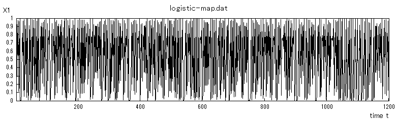
(1) ロジスティック写像
これについては、既に第1章 1.2.1 節で紹介したように、背後の力学はそこでの (21) 式で表され る1次元非線形差分方程式で記述される。また、それにより発生させた 1200時点の1次元時系列を再 掲載するとつぎのようである:
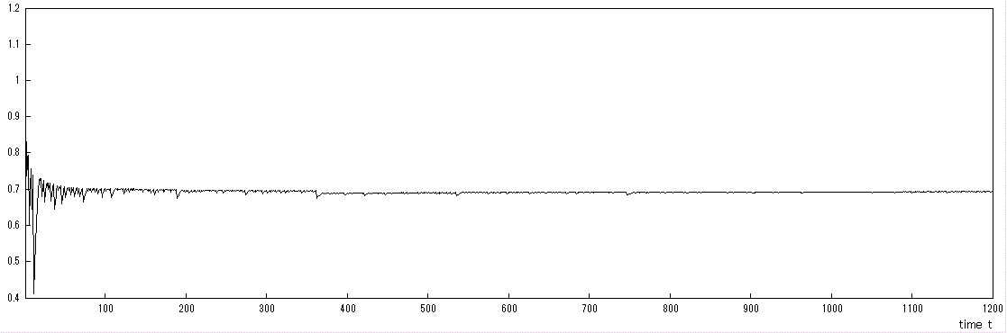
この1次元時系列を埋め込みパラメータの分析なしで3次元空間に埋め込みリアプノフ 指数を計算したが、このような分析は無理があり、そこでも述べたように3次元空間に埋め込むと最大 リアプノフ指数は理論的な真値 ln 2、すなわち、およそ 0.693476 (例えば、Sprott, 2003) にはならず (第1章 1.2.2 節 図6参照)、 最初から1次元空間に埋め込む必要があった。図2は、ロジスティック写像 データの埋め込み次元を1とした時の、リアプノフ指数を示す。ここでのリアプノフ指数計算に際しては 近傍数は 20 とした。近傍数をいろいろ変えて得られるリアプノフ指数の平均は、およそ理論値と一致し た。
なお、そのような場合、Sunday Chaos Times では、最初から埋め込み計算を行わず、リカレンスプロット、 相関積分、N 近傍プロット、...、と分析を進めればよい。この時、埋め込み計算窓で default で表示され ている「次元」3は、無視すればよい。
ここでは、このデータに対して Kennel et al. (1992) の誤り近傍法と Fraser and Swinney (1986) の 最小相互情報量を適用してみた。まず、前者の結果は図3の通りである:
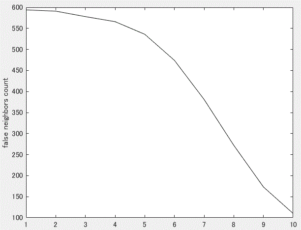
この図からは、当該データの埋め込み次元数は10以上必要であることになり、、背後の力学系が1次元 であることと矛盾する。背後の力学系が1次元とわかっている場合には Kennel et al. (1992) の誤り近傍法を使っても、適切な埋め込み次元数を推定できないことが明らかである。
ただし、われわれが手にする観測1次元時系列の背後にある力学系の次元数はわからない場合が多い。 そのような場合、万が一同データの背後にある力学系の次元数が1であれば、この例からも明らかなように、 次元数推定のための有力な方法の1つである Kennel et al. の誤り近傍法では適切な次元数を推定できない 場合がある点に注意が必要である。この問題を回避するには、われわれは手にした観測1次元時系列を生成 している背後の力学系について、当該現象が生起するメカニズムに対する理論やモデルを構築する必要があ るように思われる。この視点からは、Miao et al. (2009) は脈波の1次元観測時系列についての詳細な多次 元の力学系モデルを構築したよい例と言えるであろう。
つぎに、同一データに対して Fraser and Swinney (1986) の最小相互情報量を計算した結果を示す。図4は、 次元数2の場合の最小相互情報量の計算結果である。
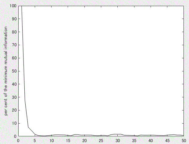
上図から、同データに対する2次元の場合の遅延増分τの推定値は8であることがわかる。ちなみに、 次元数を3から7まで上げていくと、τは6(3次元から5次元)、3(6次元)、6(7次元)となった。 いずれにせよ、ロジスティック写像データの場合、誤り近傍法の場合と同様、遅延増分の推定値はτ=1 に 比して非常に大きな値として推定されてしまう。つまり、ロジスティック写像のような 1次元写像の場合、遅延増分についても、相互情報量の計算によっては適切な値を推定できないこと になる。
(2) エノン写像
これについては、既に第1章 1.2.3 節で紹介したように、背後の力学はそこでの (22) 式で表され る2次元非線形差分方程式で記述される。なお、そこでは時点数は 1000 であったが、ここでは 3000 時点 のデータを発生させた。図5はこれを示す:
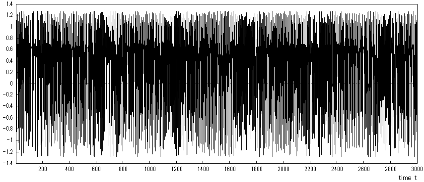
つぎに、このデータに対して Kennel et al. (1992) の誤り近傍法と Fraser and Swinney (1986) の 最小相互情報量を適用してみた。まず、前者の誤り近傍法をこのデータに適用する。ここでの遅延増分τ は、1から6まで変えた。図6はτ=1 の場合を示す:
.gif)
図6から明らかなように、エノン写像の場合、差分写像なので Cao (1997) によれば遅延増分は1が最適の はずであるが、この値で誤り近傍法を適用すると、同写像の真の次元数2では誤り近傍のパーセントは約 70 %もあり、Kennel らの基準の1%に遠く及ばない。彼らの基準からはτ=6 でようやく満たされる が、この場合推定次元数は6もしくは7となる。
いずれにせよ、ロジスティック写像の場合と同様、エノン写像の場合も、Kennel らの誤り近傍法は 真の次元数を適切に推定できないことがわかる。ただし、誤り近傍数の変化の特徴からは、図6から明らかな ように、彼らの方法でも次元数が2で誤り近傍数はエルボーを形成しており、近傍数の小ささにこだわらなけ れば、何とか次元数2を推定できているとも見れるかもしれない。
AIHARA Electrical Engineering Co., Ltd. (2002). Sunday Chaos Times. R&D Team.
Aizawa, Y., & Kohyama, T. (1984). Asymtrotically non-stationary chaos. Progress of Theoretical Physics,71,847-850.
Box, G. E. P. & Jenkins, G. M. (1970, 1976). Time series analysis: Forecastingand control. San Francisco: Holden-Day.
Cao, L. (1997). Practical method for determining the minimum embedding dimension of a scalar time series. Physica D,110, 43-50.
Casdagli, M. C. (1997). Recurrence plots revisited. Physica D,108, 12-44.
Chialvo, D. R., Gilmour, R. F., Jr, & Jalife, J. (1990). Low dimensional chaos in cardiac tissue. Nature, 343, 653-657.
Chino, N. (2002). Complex space models for the analysis of asymetry. In S. Nishisato, Y. Baba, H. Bozdogan, & K. Kanefuji (Eds.) Measurement and Multivariate Analysis, Tokyo: Springer. pp.107-114.
千野直仁 (2008). 集団のシステム解析ー微分・差分方程式モデルー 岡林春雄編著 心理学 におけるダイナミカルシステム理論 第7章 (pp.119-150). 金子書房
Chino, N. (2014). A Hilbert state space model for the formation and dissolution of affinities among members in informal groups. Supplement of the paper presented at the workshop on Problem Solving through the Applications of Mathematics to Human Behaviors by the aid of The Ministry of Education, Culture, Sports, Science and Technology in Japan, 1-24.
Chino, N. (2015). A simulation study of a Hilbert space model for changes in affinites among members in informal groups. Journal of the Institute for Psychological and Physical Science,7.
千野直仁 (2015). 正弦波時系列の 間引きによる解軌道の特徴について 研究ノート(力学系信号の間引きについての一考察)
Chino, N. & Shiraiwa, K. (1993). Geometrical structures of some non-distance models for asymmetric MDS. Behaviormetrika, 20, 35-47.
Eckmann, J. -P., Olliffson Kamphorst, S., & Ruelle, D. (1987). Recurrence plots of dynamical systems. Europhysics Letters,4,973-977.
Fraser, A. M. & Swinney, H. (1986). Independent coordinates for strange attractors from mutual information. Physical Review A, 33, 1134-1140.
Friedman, J. H., Bentley, J. L., & Frinkel, R. A. (1977). An algorithm for finding best matches in logarithmic expected time. The Association for Computing Machinery Transactions on Mathematical Software, 3, 209-226.
Gautama, T., Mandic, D. P., & Van Hulle, M. M. (2003). A differential entropy based method for determining the optimal embedding parameters of a signal. IEEE International Conference on Acoustics, Speech and Signal Processing, VI29-32.
Guillemin, V. & Pollack, A. (1974). Differential Topology, New Jersey: Prentice Hall.
Guevara, M. R., Glass, L., & Shrier, A. (1981). Phase locking, period-doubling bifurcations, and irregular dynamics in periodically stimulated cardiac cells. Science, 214, 1350-1353.
Hamilton, J. D. (1994). Time series analysis. Princeton: Princeton University.
Hannan, E. J. (1988). The statistical theory of linear systems. New York: Wiley.
Hayashi, H., Ishizuka, S., Ohta, M., & Hirakawa, K. (1982). Physics Letters, 88A,435-438.
寶来俊介、山田泰司、合原一幸 (2002). 同方向リカレンスプロットによる決定論的解析 電学論 C,122, 141-147.
日野幹雄 (2013). スペクトル解析 新装版 朝倉書店
平田祥人 (2011). リカレンスプロット:時系列の視覚化を超えて 数理解析研究所講究録 1768, 150-162.
Ikeguchi, T., & Aihara, K. (1997). Lyapunov spectral analysis on random data. International Journal of Bifurcation and Chaos, 7, 1267-1282.
Kalman, R. E. (1960). A new approach to linear filtering and prediction problems. Transactions of the ASME-Journal of Basic Engineering, 82, 35-45.
Kennel, M. B., Brown, R., and Abarbanel, H. D. I. (1992). Determining embedding dimension for pahse-space reconstruction using a geometrical construction. Physical Review A, 45, 3403-3411.
Kohyama, T. (1984). Non-stationarity of chaotic motions in an area preserving mapping. Progress of Theoretical Physics,71,1104-1107.
Lorenz, E. N. (1963). Deterministic nonperiodic flow. Journal of the Atmospheric Sciences,20,130-141.
Manneville, P. (1980). Intermittency, self-similarity and 1/f spectrum in dissipative dynamical systems. Journal de Physique,41,1235-1243.
Manneville, P., & Pomeau, Y. (1980). Different ways to turbulence in dissipative dynamical systems. Physica D,1,219-226.
May, R. (1976). Simple mathematical models with very complicated dynamics. Nature, 261, 45-67.
Mees, A., Aihara, Adachi, M., Judd, K., Ikeguchi, t., & Matsumoto, G. (1992). Deterministic prediction and chaos in squid axon response. Physical Letters, A 169、41-45.
Miao, T., Shimoyama, O., Oyama-Higa, M. (2006). Modelling plethysmogram dynamics based on baroreflex under higher cerebral influences. 2006 IEEE Conference on Systems, Man, and Cybernetics, October, Taipei, Taiwan.
Mishali, M., & Edlar, Y. C. (2009). Blind multiband signal reconstruction: Compressed sensing for analog signals. IEEE Transactions on Signal Processing, 57, 993-1009.
Molenaar, P. C. M. (2003). http://hhd.psu.edu/media/dsg/files/StateSpaceTechniques.pdf, December 31, 2015.
Noakes, L. (1991). The Takens embedding theorem. International Journal of Bifurcation and Chaos. 1, 867-872.
Nyquist, H. (1928). Certain topics in telegraph transmission. Transactions of the American Institute of Electrical Engineers. 47, 617-644.
Oseledec, V. I. (1968). A multiplicative ergodic theorem. Ljapunov characteristic numbers for dynamical systems. Transactions of the Moscow Mathematical Society, 19,197-231.
Sano, M. & Sawada, Y. (1985). Measurement of the Lyapunov spectrum from a chaotic time series. Physical Review Letters,55,1082-1085.
Shannon, C. E. (1949). Communication in the presence of noise. Proceedings of the Institute of Radio Engineers, 37, 10-21.
Schuster, H. G. (1988). Deterministic Chaos: an introduction. New York: Wiley.
Takens, F. (1981). Detecting strange attractors in turbulence. In D. A. Rand and B. S. Young, (Eds.), Dynamical Systems of Turbulence, Vol. 898 of Lecture Notes in Mathematics (pp.366-381). Berlin: Springer-Verlag.
The MathWorks, Inc. (2018). MATLAB, R2018a. Massachusetts: The MathWorks, Inc.
Tsuda, T., Tahara, T., Iwanaga, I. (1992). Chaotic pulsation in capillary vessels and its dependence on mental and physical conditions. International Journal of Bifurcation and Chaos, 2, 313-324.
上田哲生・谷口雅彦・諸澤俊介 (1995). 複素力学系序説 培風館
山田泰司、合原一幸 (1999). リカレンスプロットと2点間距離分布における非定常時系列解析 電子情報通信学会論文誌、J82A, 1016-1028.
Yule, G. U. (1927). On a method of investigating periodicities in disturbed series, with special reference to Wolfer's sunspot numbers. Philosophical Transactions of the Royal Society of London, Series A,226,267-298.
Voss, R. F. & Clarke, J. (1977). '1/f noise' in music and speech. Nature, 258, 317-318.
Webber, C. L. Jr., Zbilut, J. P. (1994). Dynamical assessment of physiological systems and states using recurrence plot strategies. Journal of Applied Physiology, 76,965-973.
Welch, P. D. (1967). The use of fast fourier transform for the estimation of power spectra: A method based on time averaging over short, modified periodograms. IEEE transactions on Audio and Electroacoustics,15,70-73.
![]()